A unified method for neural network compression

For my master’s thesis, I studied how to run deep learning models on embedded hardware, especially FPGAs with limited memory and compute. I combined three compression methods—quantization, pruning, and low-rank approximation—in one training loop.

Instead of tuning each method on its own, the network learns bit widths that also decide what to prune and whether a low-rank factorization is worth keeping. The goal was simple tuning and high compression tied directly to FPGA costs.

The three compression techniques

1. Quantization

Quantization stores weights and activations with fewer bits ($b$). This uses less memory and replaces floating-point work with cheaper integer operations. On an FPGA, both changes reduce hardware cost.

The canonical symmetric uniform quantization formula is:

$$Q(x) = \text{clamp}\left(\left\lfloor \frac{x}{S} \right\rceil, \tau_l(b), \tau_h(b)\right), \quad S = \frac{\beta - \alpha}{2^b - 1}$$

Here, $S$ is the scale set by the clipping bounds $\alpha$ and $\beta$. The limits $(\tau_l, \tau_h)$ define the integer range for $b$ bits.

In my variant, $b$ remains a trainable floating-point value. An element is pruned when its bit width falls below a threshold $\varepsilon$:

$$x_q = \alpha \cdot Q_b\left(\frac{x}{\alpha}\right), \quad Q_b(x) = \begin{cases} \text{clamp}(\lfloor x \rceil, \tau_l(b), \tau_h(b)), & b \ge \varepsilon \\ 0, & b < \varepsilon \end{cases}$$

This lets training change the compression level gradually instead of jumping between integer bit widths. Lower values make storage and arithmetic cheaper, but also leave fewer levels with which to represent the original weights.

2. Pruning

Pruning removes parameters that contribute least to the prediction.

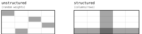
• Unstructured pruning removes individual weights. It can create high sparsity, but hardware rarely uses that sparsity well.
• Structured pruning removes whole neurons, channels, or filters. This changes tensor shapes and can produce real FPGA speedups.

Common criteria include magnitude ($L_p$) norms and APoZ (Average Percentage of Zeros).

3. Low-rank approximation

Low-rank approximation splits a large weight tensor into smaller ones with a method such as SVD. For an $m \times n$ matrix, a rank-$k$ factorization reduces the parameter count and multiply-adds from $mn$ to $k(m+n)$ when $k \ll \min(m,n)$.

The three methods change different parts of the same layer. The estimate below shows how their costs combine: pruning changes the number of output channels, rank changes the two factor matrices, and quantization changes the bits stored per weight. It is a dimensional estimate, not a trained model.

Interactive estimate

Compress a toy 64 × 64 layer

Compression settings

Weight precision

4 bits

Structured pruning

25% · 48 kept

Factorization rank

12

Parameters1,34432.8% of original

Weight storage4.1%relative to FP32

Estimated BOPS1.0%relative to FP32

Cost calculation

Compressed parameters12 × (64 + 48) = 1,344

Estimated BOPS1,344 × 4 × 8 = 43,008

BOPS holds activation precision at 8 bits. This estimates cost, not accuracy; viable settings still have to be learned and evaluated.

Why use one training objective?

The demo exposes three independent controls for intuition. My method was about avoiding that independent tuning during training. Applying the techniques separately creates two problems: their order changes the result, and each method adds hyperparameters to tune.

I first treat rank selection as structured pruning after factorization. I then treat structured pruning as low-granularity quantization. Trainable bit widths become the shared control for all three methods.

The unified objective is:

$$\min_\theta (1-\lambda) \mathcal{L}(\theta; x, y) + \lambda R(\theta_B)$$

Here, $\theta$ contains the model parameters, $\theta_B$ contains the trainable bit widths, and $\lambda$ controls the balance between task accuracy and compression. The polarization regularizer is:

$$R(B) = \gamma\lvert B\rvert_2 + t\lvert B\rvert_1 - \lvert B - \bar{B}\rvert_1$$

In this equation, $B$ is the vector of bit widths and $\bar{B}$ is its mean. The regularizer pushes unimportant elements toward zero and groups the rest away from zero. This creates a clear split between what to drop and what to keep.

This matters on FPGAs because cost scales with bit width. I estimate a layer’s cost in bit operations (BOPS) as:

$$\text{BOPS}(l) = \text{FLOPS}(l) \cdot b_w \cdot b_a$$

Learning the weight and activation widths, $b_w$ and $b_a$, while pruning the network therefore targets hardware cost directly.

The unified pipeline

1. Decompose candidate layers to expose lower-rank options.
2. Train with floating-point bit widths and the polarization regularizer.
3. Prune structures whose bit width falls below $\varepsilon$.
4. Recompose a layer if its remaining rank makes factorization more expensive than the original layer.
5. Choose one integer bit width per layer, freeze it, fine-tune the model, and deploy it.

Challenges

The bit-width penalty was the hardest part to tune. If it was too weak, the model did not compress. If it was too strong, the model collapsed and lost accuracy. I used parameter sweeps to find a useful balance between task loss and compression.

Results

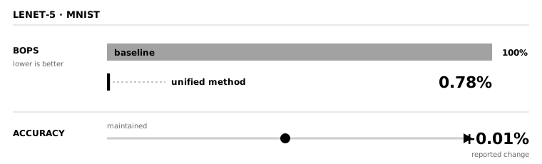
On LeNet-5 with MNIST, the method used about 0.78% of the original BOPS while accuracy rose by 0.01 percentage points. On VGG-7 with CIFAR-10, it remained competitive with mixed-precision baselines.

Summary

• Quantization lowers precision, pruning removes parameters, and low-rank approximation splits expensive layers.
• Trainable bit widths and polarization control all three methods in one objective.
• BOPS connects this objective to FPGA cost and avoids a long, order-dependent pipeline.

Patent

I did this work with my internship supervisor, Benoit Porteboeuf. It led to a published patent application for the unified compression method. The application covers the sequence of decomposition, learned quantization, pruning, optional recomposition, and fine-tuning for resource-constrained hardware.

• Published patent application WO2025051862A1