A common ML pipeline trains a model in Python, saves it, starts a model server, and moves data between that server and a database.
This works, but it adds network calls and another service to maintain. I built SQLGBM for cases where that service is not needed.
How gradient boosting works
Gradient boosting builds decision trees in sequence. Each new tree learns from the errors left by the trees before it.
The model starts with a base score and adds the output of each tree. For binary classification, a function such as the sigmoid turns the final score into a probability.
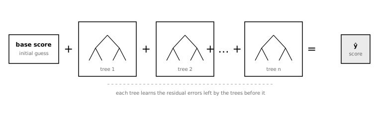
The training math is complex, but inference is simpler: each tree is a set of if-then rules.
The insight
For one row, each tree follows one decision path to a leaf. The model then adds the leaf values from all trees.
SQL can express the same logic with nested CASE statements. This means the database can run the model where the data already lives.
The toy example below keeps both representations visible. Change the row, and the highlighted path, leaf value, SQL branch, and probability all update together.
Interactive example
Follow one row from tree to SQL
Input row
42 > 35 → 68 ≤ 90 → leaf +0.65
Generated SQL sigmoid(−0.25 + 0.65) = 59.9%
1 / (1 + EXP(-(
  -0.25 +
  CASE
    WHEN age <= 35 THEN
      CASE WHEN income <= 55 THEN -0.80
           ELSE 0.35 END
    ELSE
      CASE WHEN income <= 90 THEN 0.65
           ELSE -0.15 END
  END
))) AS probability
A real boosted model repeats this traversal for every tree, adds all the leaf values to the base score, and applies the model’s link function. The generated query is larger, but the mapping is the same.
What SQLGBM does
SQLGBM automates that mapping for a trained LightGBM or XGBoost binary classifier.
First, train the model as usual.
clf = lgb.LGBMClassifier(n_estimators=100, max_depth=5)
clf.fit(X, y)
Then convert it to SQL.
from sqlgbm import SQLGBM
sqlgbm = SQLGBM(clf, X=X)
sql = sqlgbm.generate_query('my_table', 'probability')
The generated query adds one nested CASE expression per tree, sums their outputs, and applies a sigmoid. At prediction time, it runs in a compatible SQL engine without a Python runtime or model server.
Why this is useful
This approach is most useful when the features already live in a database.

For batch scoring, one query can replace exporting rows, calling an API, and writing the results back.
For online scoring, the query can be part of a view or stored procedure, depending on the database.
This can cut latency by removing serialization and network calls. It also removes a separate deployment to operate.
Tradeoffs
This only fits some use cases.
Trees map cleanly to CASE statements; neural networks map less cleanly. Large or deep ensembles also create huge queries that some engines may struggle to plan or run. SQLGBM does not yet optimize its output for each database.
Multiclass classification is not supported, and the API is still early. The project is not ready for production use.
It is best suited to simple binary classification tasks where the data is already in SQL and a model server would be overkill.
Summary
ML inference does not always need its own service. SQLGBM turns LightGBM and XGBoost trees into CASE expressions and runs them next to the data. The result is less data movement and less infrastructure for the cases it supports.
Check it out on GitHub.